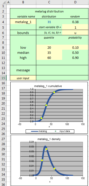
User Input Cells. Light yellow cells are user inputs. Light green cells should generally not be changed or overwritten. Later you will change the light-yellow cells to correspond to your desired input distribution. But for now, let's explore the SPT metalog distributions using the illustrative numbers provided.
Parameters and Graphs. SPT metalog distributions are parameterized by low, median, and high quantiles and by a low probability. The high probability is automatically calculated as one minus the low probability. The median probability is 0.5 by definition. Note that these probabilities are symmetric around the median. But the quantiles need not be symmetric, so skewed distributions can result. The yellow dots on the cumulative graphic show the inputs graphically. The blue curve shows the corresponding metalog distribution, which always runs exactly though these three points. The blue curve on the density graphic is the exact density that corresponds to this cumulative, and its yellow dots show where the input quantiles fall on that curve. Note that these graphs are not simulation outputs. They are graphs of the input distributions from which the SIPMath simulation will later draw its samples.
Exploring Shape Flexibility. Now let's try some different inputs to provide you with a feel for shape flexibility of metalog input distributions. The input quantiles of 20, 35 and 60 produce a right-skewed distribution because 35 is closer to 20 than to 60. Try changing the median from 35 to 40, and you'll see the metalog adjust to produce a symmetric distribution. Change the median from 40 to 50 and the metalog becomes left-skewed.
Messages and Shape-Flexibility Limits. While the metalog can produce a wide range of skewed distributions, it cannot produce infinitely skewed distributions. There's a limit. To explore this limit, reset your model to the original parameters of 20, 35, and 60 and low probability of 0.1. Then change the median to 25. A message appears to inform us that, given 10%/90% quantiles of 20 and 60, the smallest feasible median is 26.66. (Generally, messages appear as needed to provide guidance for correcting invalid inputs. If the inputs are valid, the message box remains blank.) Now change the median to 26.67, and you'll see the most right-skewed distribution available. Try other values for the median from 26.67 up to 53.33 to see the full range of left- and right-skewed shapes available.
Bounds. Metalog distributions offer four options for boundedness: unbounded (u), semi-bounded with lower bound (sl), semi-bounded with upper bound (su), and bounded (b). To explore these options, reset your template to the original parameters of 20, 35, and 60 and low probability of 0.1. Note that with a u in D6, the metalog is unbounded and the tails extend below zero and above 100. But if the uncertain variable is a market share (or any other percentage), we'd likely prefer that our metalog have lower and upper bounds of 0 and 100 respectively. To accomplish this, while maintaining the other quantile/probability parameters, simply change the u setting in D6 to b. Note that, as shown on the right, lower and upper bound input cells appear in the template, and a message informs us that we must enter bounds information. Enter 0 and 100 for the lower and upper bounds and we see that our metalog is now bounded accordingly. We can set these bounds to anything we want. For example, try changing the lower and upper bounds to 10 and 150 respectively.
Variable Name and Graph Titles. We can change the name of our uncertain variable in B4 according to our application, and the graph titles will change accordingly. For example, try changing the variable name in B4 to "market_share" and you'll see that the graph titles change accordingly. The graph titles are hidden in C15:D15. If you prefer different titles, modify these cells.
Modeling and Simulation. Once you've set your quantile, probability, bounds, and variable-name inputs to effectively represent your uncertain variable, go ahead and use this uncertain variable anywhere you like in your model, just as you would for any other uncertain variable in SIPmath, simply by referencing the distribution cell C4. The random number in D4 and Start Variable ID (random number seed) in D5 function just as they do for other SIPmath input distributions. If you wish for your metalog-distributed uncertainty to be a simulation output, select C4, click the Define Outputs command on the SIPmath toolbar, enter B4 as the variable name, and click OK. You will see that your output has been defined, just like other SIPMath output uncertainties, as shown on the bottom right, and that it also appears on the PMTable worksheet.
Moving or Rearranging the Template. To move part or all of the template (including graphics) to any other place in your workbook, or to rearrange the template, use the standard Cut (Ctrl-X) and Paste (Ctrl-V) commands. Everything will still work so long as you are pasting into blank unformatted cells. If you want the graphics to appear in more than one place, select them, and use Copy (Ctrl-C) and Paste (Ctrl-V) to copy them into an additional location.
|
 |
| Unbounded Metalog Template |
|
|