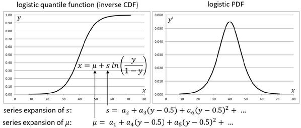
The metalog distribution (short for "meta-logistic" distribution) is derived by substituting series expansions in terms of cumulative probability y for the location and scale parameters of the logistic quantile function.
These substitutions enable virtually unlimited shape flexibility in terms of the coefficients thus introduced, and the linearity of the metalog quantile function in terms of these coefficients enables closed-form fitting to data with linear least squares.
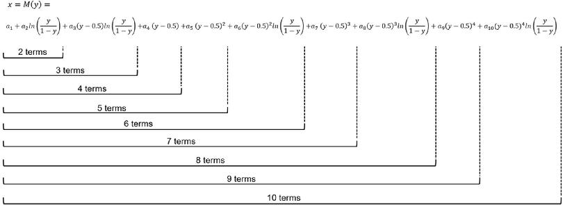
Like a Taylor series, the metalog quantile function M(y) may have any number of terms. Each additional term defines a different probability distribution and adds shape flexibility: an n-term unbounded metalog has n-2 shape parameters. While there is no limit the number of terms, practical applications typically use 2-16 terms. Given the four choices of boundedness for metalogs (unbounded, semi-bounded lower, semi-bounded upper, and bounded) and typical choices of terms from 2-16, there are approximately 60 practical distributions within the metalog system.
Unbounded metalog equations for 2-10 terms, where x is the variable of interest and y is cumulative probability.
For more detail, the metalog equations are further documented with the links below. Before examining them, you may wish to review thenotation and conventionsused throughout the metalog system. Click on a link below to see the relevant equations.
Each set of equations includes the metalog quantile function, the metalog PDF, and also a feasibility condition that must be satisfied in order for these equations to yield a valid probability distribution. See feasibility for detail (including closed form conditions for three- and four-term metalogs) and The Metalog Distributions, Section 3, Equations (5) and (10) for the derivation.
Website copyrighted by Tom Keelin 2016-2022. Free use of this website is encouraged,
including use of downloadable files. Contact: tomk@keelinreeds.com.